ABSTRACT
Modern control systems, like controllers for swarms of quadrotors, must satisfy complex control objectives while withstanding a wide range of disturbances, from bugs in their software to attacks on their sensors and changes in their environments. These requirements go beyond stability and tracking, and involve temporal and sequencing constraints on system response to various events.
This work formalizes the requirements as formulas in Metric Temporal Logic (MTL), and designs a controller that maximizes the robustness of theMTL formula. Formally, if the system satisfies the formula with robustness r, then any disturbance of size less than r cannot cause it to violate the formula. Because robustness is not differentiable, this work provides arbitrarily precise, infinitely differentiable, approximations of it, thus enabling the use of powerful gradient descent optimizers.
Experiments on a temperature control example and a two-quadrotor system demonstrate that this approach to controller design out per-forms existing approaches to robustness maximization based on Mixed Integer Linear Programming and stochastic heuristics. Moreover, it is not constrained to linear systems.
CONTROLLING FOR ROBUSTNESS
The errors in a cyber-physical control system like an automated air traffic controller can affect both the cyber components (e.g., software bugs) and physical components(e.g., sensor failures and attacks) of a system. Under certain error models, like a bounded disturbance on a sensor reading,a system can be designed to be robust to that source of error. In general, however, unforeseen and unmodeled issues will occur and the controller has to deal with them at runtime.
To help deal with unforeseen problems at runtime, the system’s controller must make decisions that not only satisfy the system’s requirements (like a maximum response time to an event), but satisfy them robustly. Intuitively, the requirements are robustly satisfied if a disturbance to the system does not cause it to violate them. This can give a margin of maneuvarability to the system during which it addresses the unforeseen problem. Since these problems are, by definition, unforeseen and unmodeled and only detected by their effect on the output, the notion of robustness must be computable using only the output behavior of the system.
ROBUSTNESS OF MTL FORMULAE
A. Metric Temporal Logic (MTL):
The controller of H is designed to make the closed loop system satisfy a specification expressed in MTL. Formally, let AP be a set of atomic propositions, which can be thought of as point-wise constraints on the state of the system.
Robust Semantics of MTL:
Designing a controller that satisfies the MTL formula φ 1 is not always enough. In a dynamic environment, where the system must react to new unforeseen events, it is useful to have a margin of maneuverability. That is, it is useful to control the system such that we maximize our degree of satisfaction of the formula. When unforeseen events occur,the system can react to them without violating the formula. This degree of satisfaction can be formally defined and computed using the robust semantics of MTL.
APPROXIMATION AND CONTROL
We implemented the smooth approximation to the semantics of MTL, and tested it on several example.
A. Approximation Error:
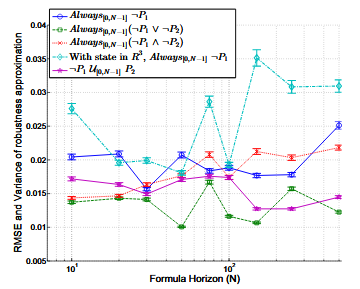
We evaluated the robustness ρ φ and its approximation ̃ρφ for five formulae. The horizon N of each formula is varied, and at each value of N we generate 1000 trajectories of system xk+1 = xk+uk with input and state saturation, by feeding it random input sequences. Fig. 1 shows the Root Mean Square (RMSE) of the approximation, √(1/1000)∑x(ρφ(x)− ̃ρφ(x))2 , and variance bars around it.

Robustness Approximation Error Against Formula Horizon, Evaluated on 1000 Randomly Generated Trajectories for Example 2. Unless Noted, the Systems are 2d. Color in Online Version
B. Robustness Maximization for Control:
Problem Pρ given in (2) is solved by replacing the true robustness ρφ by its smooth approximation ̃ρ φ, and setting min to the value of the smooth approximation error. We thus obtain Problem P ̃ρ. This approach is labeled Smooth Operator(SOP).
- Optimization solver.
- Solver initialization.
- Comparisons to BluSTL.
Results:
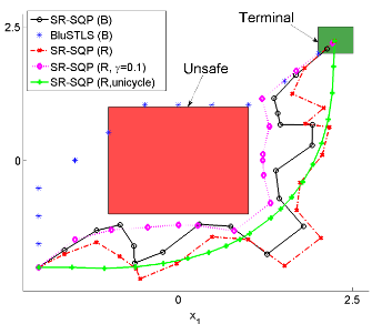
Fig 2 shows the trajectories of length N= 20 obtained by SOP and BluSTL in modes (B) and (R), starting from the same initial point x0= [−2,−2]′. Both BluSTL (B) and SOP(B) produce satisfying trajectories. The trajectory from SOP(R) ends in the middle of the terminal set, resulting in a higher robustness than mode (B), as expected.
In mode(R), BluSTL could not finish a single instance of robustness maximization within 100 hours on both the above machine and on a more powerful 8 core Intel Xeon machine with 60GB RAM, leading us to believe that the corresponding MILP was not tractable.

Fig. 2: The first 4 Trajectories are for Example 2. The Last Trajectory, SOP(R, unicycle), is from Example 3. Colors in Online Version.
Analysis:
As seen in Table I, SOP is consistently faster than BluSTL in Boolean mode, and displays smaller variances in runtimes. Note also that the problem solved here is very similar to the one used in, which uses another MILP-based method. While the underlying dynamics differ and their numbers are reported on a more power machine, SOP numbers compare favourably.
CASE STUDIES
This section focuses on evaluating the efficiency of Smooth Operator (SOP) by testing it on two systems and comparing to existing approaches.
- SOP in (B)oolean and (R)obust modes.
- BluSTL in modes (B) and (R).
- R-SQP, which uses SQP to optimize the exactnon-smoothed robustnessρφ.
- SA, which uses Simulated Annealing to optimize ρφ.
A. Hvac Control of a Building for Comfort:
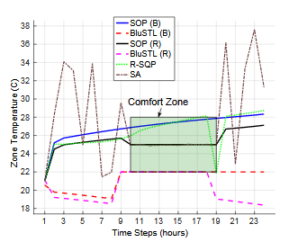
The first example is the Heating, Ventilation and Air Conditioning (HVAC) control of a 4-state model of a single zone in a building. Such a model is commonly used in literature for evaluation of predictive control algorithms. The control problem is similar to the example used. The control horizon is a 24 hour period. The objective is to bring the zone temperature to a comfortable range, Celsius, when the zone is occupied during the hours 10-to-19.

Zone Temperatures. the Green Rectangle Shows the Comfortable Temperature Limit of 22-28 C, Applicable During Time Steps 10-19 (When the Building Is Occupied). Color in Online Version.
B. Autonomous ATC for Quad-rotors:
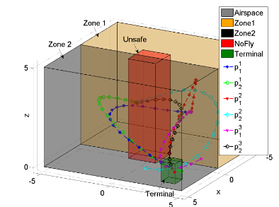
Air Traffic Control (ATC) offers many opportunities for automation to allow safer and more efficient landing patterns The constraints of ATC are complex and contain many safety rules. In this example we formalize a subset of such rules, similar to those in example 1, for an autonomous ATC for quad-rotors in MTL. We demonstrate how the smoothed robustness is used to generate control strategies for safely and robustly manoeuvring two quad-rotors in an enclosed airspace with an obstacle.
DISCUSSION AND CONCLUSIONS
We present a method to obtain smooth (infinity differentiable) approximations to the robustness of MTL formulae, with bounded and asymptotically decaying approximation error. Empirically, we show that the approximation error is indeed small for a variety of commonly used MTL formulae.
Through several examples, we show how we leverage the smoothness property of the approximation for solving a control problem by maximizing the smooth robustness, using SQP, an off-the-shelf gradient descent optimization technique. A similar approach can also be used for falsification by minimizing the smooth robustness over a set of possible initial states for a closed loop system.
We compare our technique (SOP) to other approaches for robustness maximization for control of two dynamical systems, with state and input constraints, and show how our approach consistently outperforms the other methods. While for most examples, we solve the control problem in a single-shot, finite horizon manner, in general, for a real-time implementation, the problem can be solved in an online manner as in Sec.VA.1. Future work will include a C implementation of SOP, which will allow us to experiment on real platforms, like the a fore mentioned quad-rotors, and also expand.

Trajectories Obtained via SQP on Smooth Robustness, With Three Different Initial Trajectories Acting as Initial Solutions for the SQP.
Source: University of Pennsylvania
Authors: Yash Vardhan Pant | Houssam Abbas | Rahul Mangharam