ABSTRACT
Aquaplaning accidents are relatively rare, but could have fatal effects. The task of this project is to use data from the Laser Road Surface Tester to detect road sections with risk of aquaplaning.
A three-dimensional model based on data from road surface measurements is created using MATLAB (version 6.1). From this general geometrical model of the road, a pond model is produced from which the theoretical risk ponds are detected. A risk pond indication table is further created.
The pond model seems to work well assuming that the data from the road model is correct. Determining limits for depth and length of risk ponds can be made directly by the user. MATLAB code is reasonably easy to understand and this leaves great opportunities for changing different parameters in a simple way.
Supplementary research is needed to further improve the risk pond detection model. Collecting data at smaller intervals and with more measurement points would be desirable for achieving better correlation with reality. In a future perspective, it would be wise to port the code to another programming language and this could make the computations faster.
BACKGROUND
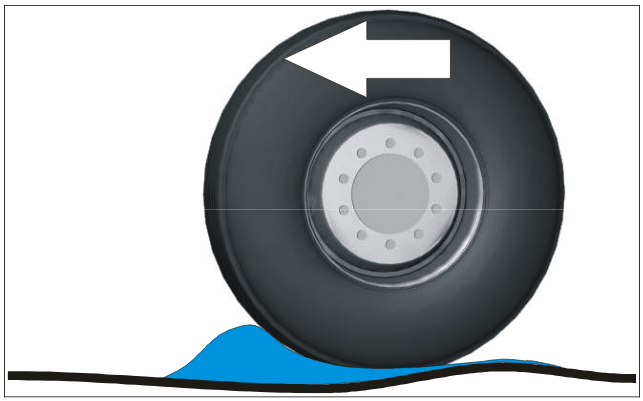
Figure 2.1. Sketch of water build-up when travelling on wet road
When a vehicle travels along a wet road, the water may accumulate and form a wedge between the road surface and the tyre. This is called water build-up and is shown in Figure 2.1. Water build-up leads to aquaplaning since water is continuously under the wheel.
![Figure 2.5. Sketch of the Laser RST with its 17 laser measurement points [39]. The numbers 0 to 16 at the bot- tom indicate the notation used for numbering the lasersFigure 2.5. Sketch of the Laser RST with its 17 laser measurement points [39]. The numbers 0 to 16 at the bot- tom indicate the notation used for numbering the lasers](http://projectabstracts.com/wp-content/uploads/2017/11/p-04569-aquaplaning-development-1.png)
Figure 2.5. Sketch of the Laser RST with its 17 laser measurement points. The numbers 0 to 16 at the bottom indicate the notation used for numbering the lasers
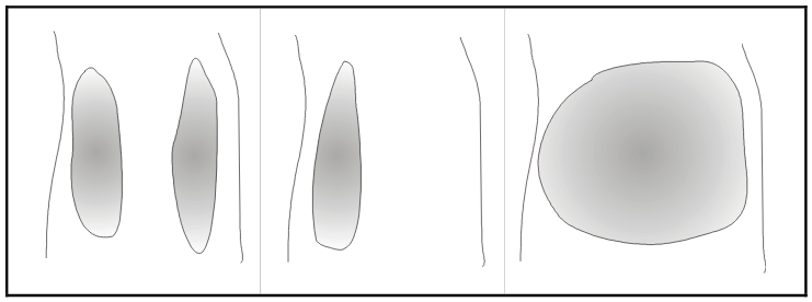
Figure 2.11. Different pond types. Left figure: Two ponds in the ruts. Middle figure: A single pond in the left rut creating asymmetrical friction. Right figure: A large pond across the whole road
Alm also reasons about the placement and size of ponds in terms of aquaplaning risk. (See Figure 2.11.) A pond situated in the middle of the road is considered to be “potentially harm- less”, whereas two symmetrical and relatively small ponds in the wheel tracks are regarded as being of minor risk. On the other hand, asymmetrical ponds across the road and large ponds at one side of the lane are considered to constitute a risk. Further, Alm discusses the properties between the depth and length of an assembly of water.
MODEL DEVELOPMENT
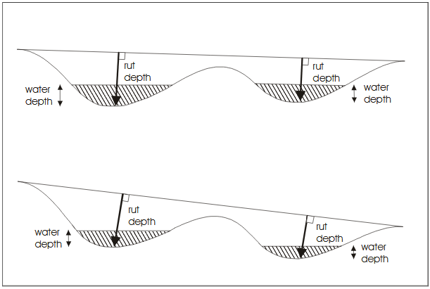
Figure 3.2. Rut depth and water depth, with (below) and without (above) crossfall. Rut depth is the same in both cases, whereas the water depth depends on the crossfall
At first sight, water depth and maximum rut depth seem to be strongly correlated. Rut depth, however, is measured according to the wire principle, as described in Subsection, and does not take crossfall into account. In Figure 3.2 the two concepts are further explained. A study by the Department of Civil and Environmental Engineering at the University of Wis-consin-Madison in the USA treated pavement rutting and safety consequences.
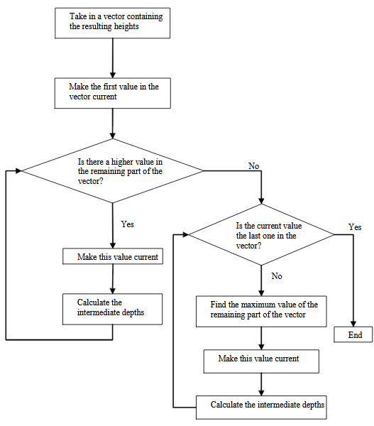
Figure 3.8. Flow chart showing the algorithm for calculating theoretical water depths for each profile from the heights
Reasoning concludes that a prerequisite of aquaplaning is that there is a possibility that water can assemble on the road. As a consequence, finding the maximum water depths at every measurement point of the road would be of great importance. This was done by first creating a depth-algorithm, which works separately across and along the road, and then by combining the resulting depths for the complete road. The depth-algorithm takes as input a vector containing the interesting heights. Figure 3.8 below shows how the algorithm works.
VALIDATION
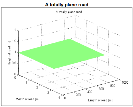
Figure 4.1. Example of a totally plane road with equal heights at 1m
To demonstrate certain features of the model, the extension of the road is sometimes chosen very small. All properties are given in metres except for crossfall, which is given in hundredths of percent. The road in Figure 4.1 is totally plane and all water is theoretically supposed to float off it. When applying the algorithm an easy validation shows that no depths are at hand for this road.
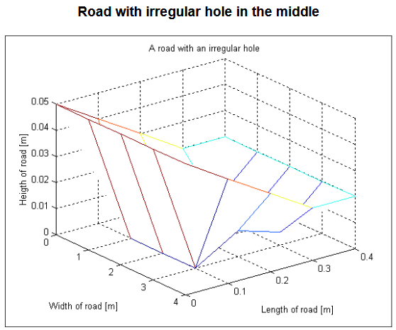
Figure 4.12. Example of a road with an irregular hole in the middle
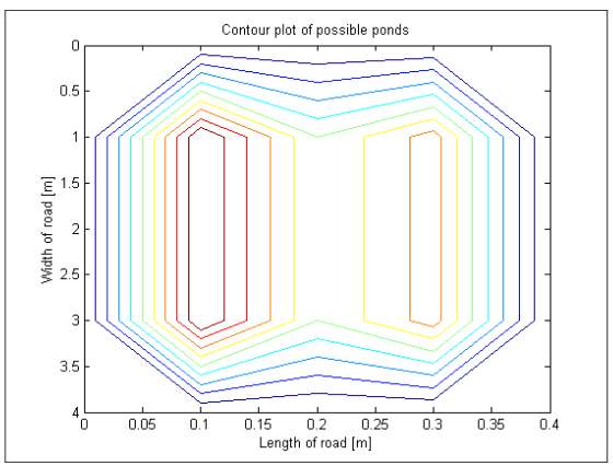
Figure 4.13. The resulting contour plot of the possible depths from the road in Figure 4.12
The road in Figure 4.12 has an irregular hole shape in the middle and the algorithm should therefore result in different water depths over the road. This can be seen in the contour plot in Figure 4.13.
DISCUSSION AND CONCLUSIONS
Model Discussion
For long road sections the calculations in the programme, especially in the pond model, are slow. It must be emphasized that the models are created in a laboratory environment and that the focus is set on completing a working model and not on execution speed at this point.
How well the road model works in reality must be proven with extensive reference measurements, which would be a too large subject to include in this master’s thesis. On one hand, the model ought to be quite good because it considers parameters collected from the roads on a basis of 17 points on a 3.2 m width and the longitudinal profiles are determined for each decimetre.
On the other hand, the mean transverse profile and crossfall are taken as an average value over a length of 20 m. The width is not the real width of the road lane, but the one measured with the survey vehicle. Additionally, the longitudinal profiles are high pass filtered and the left profile is afterwards adjusted in relation to the right in accordance with the mean transverse profile and crossfall. The system would otherwise be over-determined.
Conclusions

Figure 5.1. Flow chart showing the main steps in the progress of the work, some alternative fields of application for the road model, and for whom and what purposes the pond model may be of interest
The final summary of the development of the work can be contained in a simple flow chart, see Figure 5.1 below. The left part of the chart shows in some major steps how the work has been accomplished, whereas the right part includes some alternative areas of use for the road model, and some possible fields of application for the pond model.
Future Improvement
Further research on the aquaplaning phenomenon is needed to fully examine the problem. Most references listed in this report have their basis on experiments in a fixed environment or under not road-like conditions. Their aim has often been to compare certain types of tyres with respect to tyre tread depth, width or pattern design. The experiments have been performed at different speeds and on different grounds, but not on actual roads. Therefore, no greater confidence in the results obtained should prevail until more thorough tests have been carried out on real roads. Work that needs to be done in the future is relating actual water film thickness on the road surface and the extent of a hazardous water accumulation with the potential of aquaplaning.
Source: Linköping University
Author: Sara Nygårdhs
>> Simple Matlab Projects for EEE Final Year Students
>> Easy Microcontroller Project Ideas for Students
>> Top 50+ MATLAB based Simulation Mini Project Topics & Final Year Project Titles for ECE Students
>> Matlab Projects Fingerprint Recognition and Face detection for Final Year Students
>> 200+ Matlab Projects based on Control System for Final Year Students