INTRODUCTION
Our goal was to create a fully operational mobile application which could detect, recognize and track human faces.
In order to do that, we have decided to use the Android platform combined with the open cv library.
The development of the application was made on Qual comm MSM8960 mobile device which run a 4.0.3 Android OS.
In addition to the application we have built, we also did a research about how well we can use LDA and PCA in order to recognize faces and also about the use of LDA in order to do basic pose estimation.
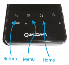
Figure 1: Qualcomm MSM8960 buttons.
Smartphone’s buttons On every android smartphone there are three buttons that you must be familiar with in order to operate our application:
- Home button.
- Return button.
- Menu button.
Smartphone’s buttons On every android smartphone there are three buttons that you must be familiar with in order to operate our application: Home button. Return button. Menu button.
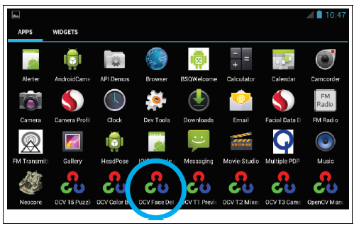
Figure 2: Launch the application.
After launching the application we will see the application:
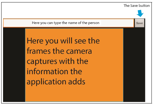
Figure 3: The application’s layout.
ANDROID AND CLASS DIAGRAM IN A NUTSHELL
As introduced, the application is written in Java as an Android application. Now, intuitively what is the “use cycle” of every mobile application?, namely, what states the application can be at? The main states the application can be at are:
- Running, it is the most essential state
- Starting for the first time since you permanently exited it
- Pausing
- Exiting
- Returning from pause
What the Android platform cleverly do is supplying an interface of methods that de ne/implement each of the above states and obligating the developer to implement each of the methods. We can see it more clearly using this chart:
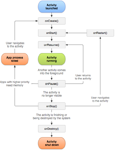
Figure 9: Activity lifecycle chart.
FACE DETECTION
We set our main ROI (Region Of Interest) to be the bounding rectangle of the face meaning by any case we do not look or do actions on the parts of the frame that are out of the boundaries of the ROI. Now we divide the face into sub-ROIs:
- ROI of the left eye
- ROI of the right eye
- ROI of the nose
- ROI of the mouth
Now we use the “detectMultiScale” method on every ROI – we give the method as parameter the image/frame that represents the part of the frame that is related to the mentioned part of face, and we give the relevant cascade for this ROI in order to detect the relevant part of the face. E.g. when we wish to nd the left eye, we set the left eye ROI, as will be described, and we use the “detectMultiScale” method on that ROI using the left eye cascade. We found out that the best parts of face ROIs division is:
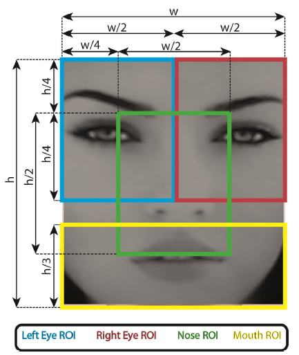
Figure 11: Relative parts of face ROI division (on a face that was detected by the first call to “detectMultiScale”).
FACE RECOGNITION
Our application supports recognition of faces of people who were recorded into the application’s data base. In this section we will explain the implementation and the ” field results” of the face recognition part in the application. This section will be a direct continuation to the “face detection” section.
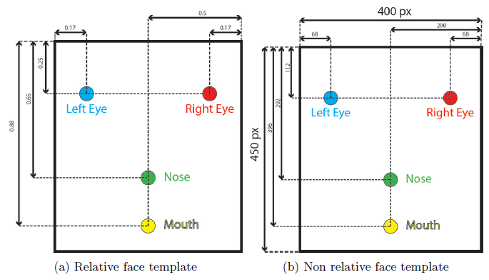
Figure 12: Face Templates.
As we already explained, the method “analyzeFrame” iterated over all the faces that were detected in the frame, and for each face the method finds the eyes, the nose and the mouth of that face. If there are no errors in the detection then we continue to the recognition part.
Now let us look at the ROC curve which represents the true positive rate and the false negative rate as a function of the threshold:
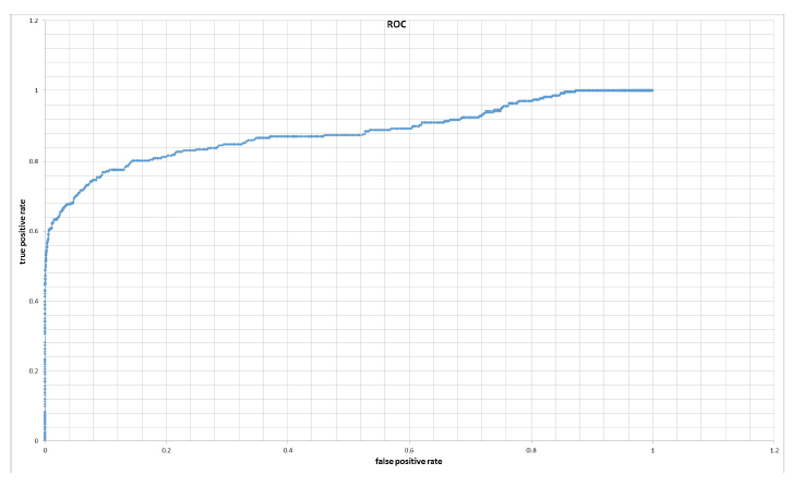
Figure 14: Threshold ROC using Chi-Square norm.
From the ROC curve we can learn that a threshold of around 290-350 can give us a TPR of 0.78-0.83 and FPR of 0.13-0.25 which is very good. The table below should detail the top left area of the ROC graph:
TRACKING
If the face that we recognized is on the list of the faces that needs to be tracked (this list is in the file “TrackingSettings.txt” and it is changed if we press on the “menu button” and then press on “tracking”) then we will start the tracking – the user will see a red bounding box around the recognized face. Whenever the recognized person tilts his face, or turns his face – the bounding box will track his face and won’t let go.
FACE RECOGNITION AND POSE ESTIMATION USING PCA AND LDA
After the failure in using only LDA we tried to rst reduce initial dataset of the histograms of size 1×16384 using PCA and only after that using the LDA. By using the “princomp” comment in Matlab we were able to reduce the his- tograms to a much lower dimension:
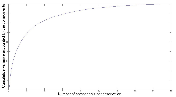
Figure 18: Cumulative variance accounted by the components as a function of the number of components.
The results were quite poor { no matter to how much dimentions we lowered the dataset, we only got separation of 53% (we mean that the best separation is a distance where 53% of the first graph are to its right and 53% of the second graph are to its left) in all the cases.
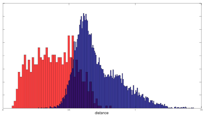
Figure 19: Probability distribution function of the distances between a pair of faces where the dimension reduction of the PCA was 23 and the dimension reduction of the LDA was 22.
When we used 23 of the PCA componenets { i.e. we reduced the LBP his- tograms from 1×16384 to 1×23 and we ran LDA on that data and reduced the data of the LDA to 22 dimensions, built the “same” “not same” graphs using the L2 norm we got 86% separation.
We wanted to check whether doing dimension reduction using only PCA could get us to good results. We extracted the LBP histograms as earlier, converted them to Matlab, ran the PCA in iterations from 1 to 172, built the “same” “not same” graphs per each iteration and checked where the separation rate of the graphs, the results are presented in the following graph:
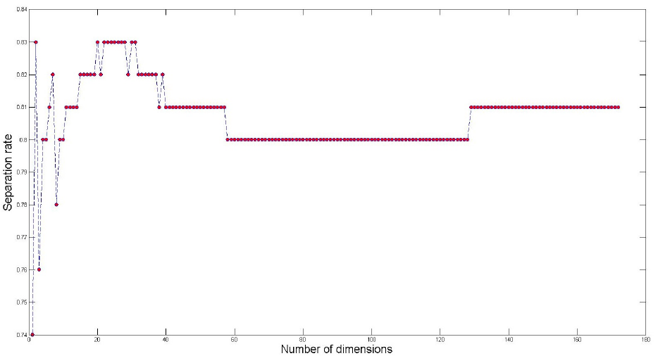
Figure 20: Separation rate as a function of the number of dimensions. The red dots are the results.
CONCLUTION
We saw that using soley LDA gives us poor results. Using soley PCA gives us much better results, and the the combination of the two gives us the best results, although not far from the results gotten by using soley PCA. All these conslusions can be seen clearly in the combined ROC graphs:
Source: Technion
Authors: Vardan Papyan | Emil Elizarov
>> Matlab Projects Fingerprint Recognition and Face detection for Final Year Students
