ABSTRACT

The fuel pressure is one of the central control variables of a modern common-rail injection system. It influences the generation of nitrous oxide and particulate matter emissions, the brake specific fuel consumption of the engine and the power consumption of the fuel pump.

Accurate control of the fuel pressure and reliable diagnostics of the fuel system are therefore crucial components of the engine management system. In order to develop for example control or diagnostics algorithms and aid in the understanding of how hardware changes affect the system, a simulation model of the system is desirable.

A Simulink model of the XPI (Xtra high Pressure Injection) system developed by Scania and Cummins is developed. Unlike the previous models of the system available, the new model is geared towards fast simulations by modelling only the mean flow and pressure characteristics of the system, instead of the momentary flow and pressure variations as the engine rotates.

The model is built using a modular approach where each module represents a physical component of the system. The modules themselves are based to a large extent on the physical properties of the components involved, making the model of the system adaptable to different hardware configurations whilst also being easy to understand and modify.

MODELING

Overview

The system was modeled in three stages, each stage attempting to capture different physical parts of the system. The first stage dealt with the low pressure part of the system, the second the HPP and the third stage the high pressure parts such as the injectors and the fuel rail. The most difficult stage was the second one-two different modelling approaches were tried in order to find a model of the pump that could capture the fuel flow accurately enough with a sufficiently low computational burden.

Some components, such as the fluid, were necessary in all three stages of the modelling process. Since these components are used frequently, they are described in the first sections of this chapter.

Low Pressure System

The first components in the fuel flow path of the system are the fuel filters, low pressure pump, regulator valve, inlet metering valve, air-bleed orifice and venturi (see figure 1.1). The models for these components will be described and motivated in the following section.

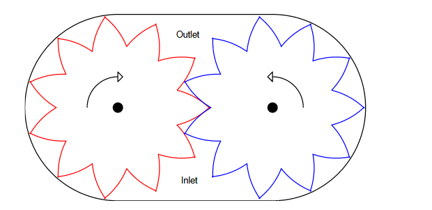
Figure 2.1. Drawing of a gear-type pump similar to the low pressure pump of the XPI system

High Pressure Pump

The most challenging part of the system to model has been the high pressure pump and its associated inlet and outlet check valves. Due to the large difference between the inlet and outlet pressures of the pump, the fluid properties and also the leakage vary greatly over the course of a pumping cycle which should be accounted for in order for the discharge rate of the pump to be correct.

MODEL VERIFICATION AND RESULTS

Low Pressure System

The main purpose of the model of the low pressure system is to generate the pressure in the control volume upstream of the ICV. That pressure is generated by the fluid flow through the IMV and other flows; since the flow through the IMV is a function of the pressure upstream of the IMV it is important that the pressure is correct. Unfortunately no direct measurement data was available for that pressure, instead the model developed by Cummins was used as a reference. That model is accurate to within 5% of actual measured data from a test rig at Cummins (e-mail correspondance with Thomas Timren, 2011-02-10). The comparison between the two models can be seen in figure 3.1.

Figure 3.1. Simulated pressure before the IMV from the GT-FUEL model developed by Cummins [25] and the Simulink model developed within this thesis as described in section 2.5

Due to the lack of measurement data, some results of the cycle modelling HPP have only been compared to the model from Cummins. In figures 3.2, 3.3, 3.4 and 3.5 the pumping chamber pressure, ICV and OCV flow rates and pump leakage as a function of the crank shaft angle relative to the initial position are compared for the GT-FUEL model from Cummins and the cycle modelling Simulink model.

Figure 3.2. Simulated pump chamber pressure from the GT-FUEL model developed by Cummins [25] and the Simulink model developed within this thesis as described in section 2.6.3

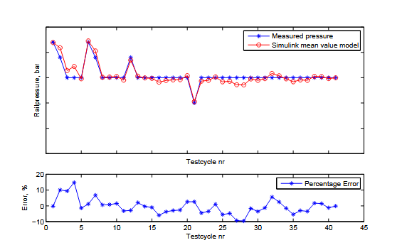
Once a complete model of the system had been assembled it was tested by stimulating it with engine speed, injection time and IMV current data from tests performed in an injection test rig. First the stationary points from appendix C were used to test the system over a broad spectrum of operating points. The results can be seen in figure 3.8; several of the tested operating points result in a simulated rail pressure more than 10% lower or higher than the true pressure. The worst point results in a rail pressure about 15% higher than the true pressure and another four are at or just outside the 10% limit.

Figure 3.8. The measured and simulated rail pressure for the different stationary points specified in appendix C. Several of the operating points result in rail pressures more than 10% higher or lower than the true rail pressure

DISCUSSION

Overview

In the following sections, some of the limitations and their causes, the models suitability for different applications and possible improvements will be briefly dis- cussed. The results of the developed model will also be related to the goals set forth in chapter 1.3.

Limitations of the Model

The current-flow area curve of the IMV, figure 2.3, imposes a severe limitation on the range of IMV currents that can be used in the model. With the available data, the entire permissible range of IMV currents could not be mapped to an effective flow area – for IMV currents outside the mapped range, linear extrapolation is used to estimate the effective area. This will most likely introduce large errors in the effective area of the IMV if the current is far outside the mapped range of currents.

Suitable Applications

Since the time constant of the model can be made to agree with measured data with relative ease, the model should be suitable for testing rail pressure control algorithms and other features that are dependent upon the time constant of the system. This could for example include high pressure leakage diagnosis or diagnosis and adaptation of large injector flows.

Suggested Improvements

As mentioned in section 3.3, the linear leakage model is a prime candidate for improvement since it displays a large error relative to the total leakage flow. The actual flow error is also large enough to make it among the larger of all the flow errors, thus reducing the leakage flow error percentage from the current ≈ 20% (figure 3.7) of the total leakage in the worst operating points to a level similar to that of the HPP inlet flow rate (figure 3.6) would make a significant difference in the total flow rate error.

Conclusion

The goal of the thesis as set forth in section 1.3 was to develop a model of the XPI system that could simulate the rail pressure as a function of engine speed, commanded IMV position and fuel injection rate. Such a model has been developed using a physical modelling approach to a large extent, unfortunately the simulated rail pressure does not meet the goal of being within 10% of the actual rail pressure in all permissible operating points of the engine. Out of 41 tested stationary operating points, one results in a rail pressure that is 15% to high and another four are at or slightly above the 10% limit. The remaining 36 points meet the requirement. When tested against dynamic rail pressure data the system displays similar performance with a maximum deviation of about 15%.

Source: Linköping University
Author: Källkvist, Kurt

Download Project

>> Simulink Projects using Matlab for Engineering Students

>> Automobile based Matlab Project Topics with Free Base Papers Downloads

>> Automobile based Projects for Final Year Students

>> Simulation based Projects for Students

>> 200+ Matlab Projects based on Control System for Final Year Students