ABSTRACT
Deep neural networks are being widely used for feature representation learning in diverse problem areas ranging from object recognition and speech recognition to robotic perception and human disease prediction. We demonstrate a novel, perhaps the first application of deep learning in mechanical design, specifically to learn complex microfluidic flow patterns in order to solve inverse problems in fluid mechanics.
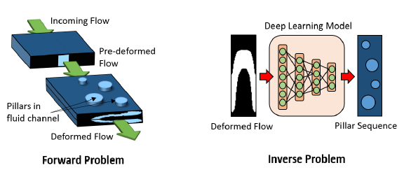
A recent discovery showed the ability to control the fluid deformations in a microfluidic channel by placing a sequence of pillars. This provides a fundamental tool for numerous material science, manufacturing and biological applications. However, designing pillar sequences for user-defined deformations is practically infeasible as the current process requires laborious and time-consuming design iterations in a very large, highly nonlinear design space that can have as large as 1015 possibilities.
We demonstrate that hierarchical feature extraction can potentially lead to a scalable design tool via learning semantic representations from a relatively small number of flow pattern examples. The paper compares the performances of pre-trained deep neural networks and deep convolutional neural networks as well as their learnt features. We show that a balanced training data generation process with respect to a metric on the output space improves the feature extraction performance. Overall, the deep learning based design process is shown to expedite the current state-of-the-art design approaches by more than 600 times.
PROBLEM SETUP

Figure 1: Illustration of the forward and the inverse problem.
One approach to solve the inverse design problem is to assign class indices to pillars with different specifications. For example, a pillar at position 0:0 and diameter 0:375 will be assigned an index of 1, whereas another pillar at position 0:125 and diameter 0:375 will be assigned an index of 2. Index assignment is performed over a finite combination of pillar positions and diameters that has been obtained by discretizing the design space. In this study, there are 32 possible indices that describes the diameter and position of a single pillar.
This formulation is applicable on both DNN and CNN architectures (CNN with SMC shown in Figure 2) and requires only a slight modification in the loss function. For an np-pillar problem, the loss function to be minimized for a data set D is the negative log likelihood defined as:

where D denotes the training set, θ is the model parameters with W as the weights and b for the biases. y is predicted pillar index whereas x is the provided ow shape test image. The total loss is obtained by summing the losses computer for each pillar.
TRAINING DATA GENERATION USING A METRIC ON THE OUTPUT SPACE
Figure 3: Uniform sampling vs. Quasi-random sampling. A set of 160 2-pillar sequences are formed using uniform (left) and Sobol (right) sampling methods. The first 10 sampled sequences are shown in red, the next 50 sampled sequences in green, and the final 100 sampled sequences in blue.
By minimizing DN (low discrepancy), the points sampled will fill the space defined by the intervals in B more evenly than uncorrelated random points (Press 1992). Thus, low discrepancy sampling helps to prevent crowding or large gaps in the selected pillar sequences, which should create a more balanced and varied dataset of pillar sequences as illustrated in Figure 3.
EXPERIMENTS AND RESULTS

Figure 4: Eight example predictions (np = 4). The left side of each pair is the target ow shape and the right side is the ow generated from the predicted pillar sequences.
After the network makes a prediction, the resulting sequence is used to generate the ow shape which is then compared with the target shape as shown in Figure 4. The pixel match rate (PMR) is used as a performance metric. In simpler terms, given an original ow shape image and an image generated from the predicted pillar sequences using the DL model, two pixels at corresponding locations match if they both have the same color.

Figure 6: Visualization of CNN lters and feature maps of a test sample from convolutional layers 1 and 2.
In CNNs, learned features can be visualized by plotting the weight matrix of the feature maps in the same manner as obtaining filter-like representations from DNNs. Figure 6 shows the filters and convolved feature maps from both convolutional layers. Filters, with corresponding feature maps, are chosen at random to reveal the edge-like features that are learned by the model.

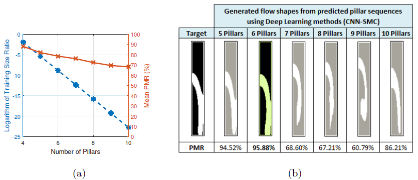
Figure 8: (a) Variation of the average PMR and training size ratio (ratio of training samples to the number of all possible pillar sequences, on a logarithmic scale) with increasing number of pillars in a sequence. (b) Flow shapes generated from predicted pillar sequences.
Figure 8 (a) shows the capability of the hierarchical model under this “curse-of-dimensionality” challenge. Even with an exponential decrease in coverage of the design space, the PMR rate only degrades linearly. Figure 8 (b) shows the ow shape generated from predicted pillar sequences based on an example input ow shape. The PMR values for this example are consistent with the results obtained from Figure 8 (a).
CONCLUSIONS
This paper proposes a deep learning based approach to solve complex design exploration problems, specifically design of microfluidic channels for ow sculpting. We have demonstrated that DL based tools can achieve the required design accuracy. The state-of-the-art GA based method performs slightly better quantitatively, but it remains a less desirable solution due very long execution time. DL based methods can expedite the design process by more than 600 times and present a real-time design alternative.
A quasi-random training data generation process was developed based on a metric on the output space. Such a process can be used for learning features from simulation and experimental data in many physical problems in general. The training data generation and hierarchical feature extraction processes together proves to be quite useful for a scalable design tool. Finally, feature visualization is performed to investigate ow pattern aspects at various scales. Current efforts are primarily focusing on optimizing the tool-chain as well as tailoring for specific application areas such as manufacturing and biology.
Source: Iowa State University
Authors: Kin Gwn Lore | Daniel Stoecklein | Michael Davies | Baskar Ganapathysubramanian | Soumik Sarkar

